Airy-Funktion

Dieser Artikel beschreibt eine spezielle Funktion. Für die Formel, die die Transmission von elektromagnetischer Strahlung beschreibt siehe Airy-Formel.

Die Airy-Funktion Ai ( x ) {\displaystyle \operatorname {Ai} (x)} bezeichnet eine spezielle Funktion in der Mathematik. Die Funktion Ai ( x ) {\displaystyle \operatorname {Ai} (x)} und die verwandte Funktion Bi ( x ) {\displaystyle \operatorname {Bi} (x)} , die ebenfalls Airy-Funktion genannt wird, sind Lösungen der linearen Differentialgleichung

  y x y = 0   , {\displaystyle \ y''-xy=0\ ,}

auch bekannt als Airy-Gleichung. Sie beschreibt unter anderem die Lösung der Schrödinger-Gleichung für einen linearen Potentialtopf.

Die Airy-Funktion ist nach dem britischen Astronomen George Biddell Airy benannt, der diese Funktion in seinen Arbeiten in der Optik verwendete (Airy 1838). Die Bezeichnung Ai ( x ) {\displaystyle \operatorname {Ai} (x)} wurde von Harold Jeffreys eingeführt.

Definition

Reelle Airy-Funktion

Für reelle Werte x {\displaystyle x} ist die Airy-Funktion als Parameterintegral definiert:

A i ( x ) = 1 π 0 cos ( t 3 3 + x t ) d t   . {\displaystyle \mathrm {Ai} (x)={\frac {1}{\pi }}\int \limits _{0}^{\infty }\cos \left({\frac {t^{3}}{3}}+xt\right)\,{\rm {d}}t\ .}

Eine zweite, linear unabhängige Lösung der Differentialgleichung ist die Airy-Funktion zweiter Art B i {\displaystyle \mathrm {Bi} } :

B i ( x ) = 1 π 0 ( exp ( t 3 3 + x t ) + sin ( t 3 3 + x t ) ) d t   . {\displaystyle \mathrm {Bi} (x)={\frac {1}{\pi }}\int \limits _{0}^{\infty }\left(\exp \left(-{\frac {t^{3}}{3}}+xt\right)+\sin \left({\frac {t^{3}}{3}}+xt\right)\right)\,{\rm {d}}t\ .}

Komplexe Airy-Funktion

Die komplexe Airy-Funktion ist

Ai ( z ) = 1 2 π i C exp ( t 3 3 z t ) d t , {\displaystyle \operatorname {Ai} (z)={\frac {1}{2\pi i}}\int _{C}\exp \left({\tfrac {t^{3}}{3}}-zt\right)\,dt,}

mit Kontour C {\displaystyle C} von z 1 = {\displaystyle z_{1}=\infty } mit arg ( z 1 ) = π / 3 {\displaystyle \operatorname {arg} (z_{1})=-\pi /3} nach z 2 = {\displaystyle z_{2}=\infty } mit arg ( z 2 ) = π / 3 {\displaystyle \operatorname {arg} (z_{2})=\pi /3} .

Eigenschaften

Asymptotisches Verhalten

Für x {\displaystyle x} gegen + {\displaystyle +\infty } lassen sich A i ( x ) {\displaystyle \mathrm {Ai} (x)} und B i ( x ) {\displaystyle \mathrm {Bi} (x)} mit Hilfe der WKB-Näherung approximieren:

A i ( x ) e 2 3 x 3 / 2 2 π x 1 / 4 B i ( x ) e 2 3 x 3 / 2 π x 1 / 4 . {\displaystyle {\begin{aligned}\mathrm {Ai} (x)&{}\simeq {\frac {e^{-{\frac {2}{3}}x^{3/2}}}{2{\sqrt {\pi }}\,x^{1/4}}}\\\mathrm {Bi} (x)&{}\simeq {\frac {e^{{\frac {2}{3}}x^{3/2}}}{{\sqrt {\pi }}\,x^{1/4}}}.\end{aligned}}}

Für x {\displaystyle x} gegen {\displaystyle -\infty } gelten die Beziehungen:

A i ( x ) sin ( 2 3 ( x ) 3 / 2 + 1 4 π ) π ( x ) 1 / 4 B i ( x ) cos ( 2 3 ( x ) 3 / 2 + 1 4 π ) π ( x ) 1 / 4 . {\displaystyle {\begin{aligned}\mathrm {Ai} (x)&{}\simeq {\frac {\sin({\frac {2}{3}}(-x)^{3/2}+{\frac {1}{4}}\pi )}{{\sqrt {\pi }}\,(-x)^{1/4}}}\\\mathrm {Bi} (x)&{}\simeq {\frac {\cos({\frac {2}{3}}(-x)^{3/2}+{\frac {1}{4}}\pi )}{{\sqrt {\pi }}\,(-x)^{1/4}}}.\end{aligned}}}

Nullstellen

Die Airy-Funktionen haben nur Nullstellen auf der negativen reellen Achse.[1] Die ungefähre Lage folgt aus dem asymptotischen Verhalten für x {\displaystyle x\to -\infty } zu

Ai ( x ) = 0 x ( 3 2 π ( n 1 4 ) ) 2 / 3 , n N {\displaystyle \operatorname {Ai} (x)=0\quad \Rightarrow \quad x\approx -{\bigl (}\textstyle {\frac {3}{2}}\pi (n-{\frac {1}{4}}){\bigr )}^{2/3},\quad n\in \mathbb {N} }
Bi ( x ) = 0 x ( 3 2 π ( n 3 4 ) ) 2 / 3 , n N {\displaystyle \operatorname {Bi} (x)=0\quad \Rightarrow \quad x\approx -{\bigl (}\textstyle {\frac {3}{2}}\pi (n-{\frac {3}{4}}){\bigr )}^{2/3},\quad n\in \mathbb {N} }

Spezielle Werte

Die Airy-Funktionen und ihre Ableitungen haben für x = 0 {\displaystyle x=0} die folgenden Werte:

A i ( 0 ) = 1 9 3 Γ ( 2 3 ) , A i ( 0 ) = 1 3 3 Γ ( 1 3 ) , B i ( 0 ) = 1 3 6 Γ ( 2 3 ) , B i ( 0 ) = 3 6 Γ ( 1 3 ) . {\displaystyle {\begin{aligned}\mathrm {Ai} (0)&{}={\frac {1}{{\sqrt[{3}]{9}}\cdot \Gamma ({\frac {2}{3}})}},&\quad \mathrm {Ai} '(0)&{}=-{\frac {1}{{\sqrt[{3}]{3}}\cdot \Gamma ({\frac {1}{3}})}},\\\mathrm {Bi} (0)&{}={\frac {1}{{\sqrt[{6}]{3}}\cdot \Gamma ({\frac {2}{3}})}},&\quad \mathrm {Bi} '(0)&{}={\frac {\sqrt[{6}]{3}}{\Gamma ({\frac {1}{3}})}}.\end{aligned}}}

Hierbei bezeichnet Γ ( ) {\displaystyle \Gamma (\cdot )} die Gammafunktion. Es folgt, dass die Wronski-Determinante von A i ( x ) {\displaystyle \mathrm {Ai} (x)} und B i ( x ) {\displaystyle \mathrm {Bi} (x)} gleich 1 π {\displaystyle {\tfrac {1}{\pi }}} ist.

Fourier-Transformierte

Direkt aus der Definition der Airy-Funktion Ai ( x ) {\displaystyle \operatorname {Ai} (x)} (siehe oben) folgt deren Fourier-Transformierte.

F ( Ai ) ( k ) := Ai ( x )   e 2 π i k x d x = e i 3 ( 2 π k ) 3 . {\displaystyle {\mathcal {F}}(\operatorname {Ai} )(k):=\int _{-\infty }^{\infty }\operatorname {Ai} (x)\ \mathrm {e} ^{-2\pi \mathrm {i} kx}\,dx=\mathrm {e} ^{{\frac {\mathrm {i} }{3}}(2\pi k)^{3}}\,.}

Man beachte die hier verwendete symmetrische Variante der Fourier-Transformation.

Weitere Darstellungen

A i ( z ) = 1 3 2 / 3 Γ ( 2 3 ) 0 F 1 ( 0 ; 2 3 ; 1 9 z 3 ) z 3 1 / 3 Γ ( 1 3 ) 0 F 1 ( 0 ; 4 3 ; 1 9 z 3 ) {\displaystyle \mathrm {Ai} (z)={\frac {1}{3^{2/3}\cdot \Gamma ({\tfrac {2}{3}})}}\cdot \,{}_{0}F_{1}\left(0;{\tfrac {2}{3}};{\tfrac {1}{9}}z^{3}\right)-{\frac {z}{3^{1/3}\cdot \Gamma ({\tfrac {1}{3}})}}\cdot \,{}_{0}F_{1}\left(0;{\tfrac {4}{3}};{\tfrac {1}{9}}z^{3}\right)}
B i ( z ) = 1 3 1 / 6 Γ ( 2 3 ) 0 F 1 ( 0 ; 2 3 ; 1 9 z 3 ) + 3 1 / 6 z Γ ( 1 3 ) 0 F 1 ( 0 ; 4 3 ; 1 9 z 3 ) {\displaystyle \mathrm {Bi} (z)={\frac {1}{3^{1/6}\cdot \Gamma ({\tfrac {2}{3}})}}\cdot \,{}_{0}F_{1}\left(0;{\tfrac {2}{3}};{\tfrac {1}{9}}z^{3}\right)+{\frac {3^{1/6}\cdot z}{\Gamma ({\tfrac {1}{3}})}}\cdot \,{}_{0}F_{1}\left(0;{\tfrac {4}{3}};{\tfrac {1}{9}}z^{3}\right)}
A i ( x ) = 1 3 x [ I 1 / 3 ( 2 3 x 3 / 2 ) I 1 / 3 ( 2 3 x 3 / 2 ) ] {\displaystyle \mathrm {Ai} (x)={\frac {1}{3}}{\sqrt {x}}\left[I_{-1/3}\left({\frac {2}{3}}x^{3/2}\right)-I_{1/3}\left({\frac {2}{3}}x^{3/2}\right)\right]}
B i ( x ) = x 3 [ I 1 / 3 ( 2 3 x 3 / 2 ) + I 1 / 3 ( 2 3 x 3 / 2 ) ] {\displaystyle \mathrm {Bi} (x)={\sqrt {\frac {x}{3}}}\left[I_{-1/3}\left({\frac {2}{3}}x^{3/2}\right)+I_{1/3}\left({\frac {2}{3}}x^{3/2}\right)\right]}
  • Eine andere unendliche Integraldarstellung für A i {\displaystyle \mathrm {Ai} } lautet
A i ( z ) = 1 2 π exp ( i ( z t + t 3 3 ) ) d t {\displaystyle \mathrm {Ai} (z)={\frac {1}{2\pi }}\int \limits _{-\infty }^{\infty }\exp \left(\mathrm {i} \cdot \left(zt+{\frac {t^{3}}{3}}\right)\right)\mathrm {d} t}
  • Es gibt die Reihendarstellungen[2]
A i ( z ) = 1 3 2 / 3 π n = 0 Γ ( 1 3 ( n + 1 ) ) n ! ( 3 1 / 3 z ) n sin ( 2 ( n + 1 ) π 3 ) {\displaystyle \mathrm {Ai} (z)={\frac {1}{3^{2/3}\pi }}\sum _{n=0}^{\infty }{\frac {\Gamma \left({\frac {1}{3}}(n+1)\right)}{n!}}\left(3^{1/3}z\right)^{n}\sin \left({\frac {2(n+1)\pi }{3}}\right)}
B i ( z ) = 1 3 1 / 6 π n = 0 Γ ( 1 3 ( n + 1 ) ) n ! ( 3 1 / 3 z ) n | sin ( 2 ( n + 1 ) π 3 ) | {\displaystyle \mathrm {Bi} (z)={\frac {1}{3^{1/6}\pi }}\sum _{n=0}^{\infty }{\frac {\Gamma \left({\frac {1}{3}}(n+1)\right)}{n!}}\left(3^{1/3}z\right)^{n}\left|\sin \left({\frac {2(n+1)\pi }{3}}\right)\right|}

Komplexe Argumente

A i ( x ) {\displaystyle \mathrm {Ai} (x)} und B i ( x ) {\displaystyle \mathrm {Bi} (x)} sind ganze Funktionen. Sie lassen sich also auf der gesamten komplexen Ebene analytisch fortsetzen.

[ A i ( x + i y ) ] {\displaystyle \Re \left[\mathrm {Ai} (x+iy)\right]} [ A i ( x + i y ) ] {\displaystyle \Im \left[\mathrm {Ai} (x+iy)\right]} | A i ( x + i y ) | {\displaystyle |\mathrm {Ai} (x+iy)|\,} a r g [ A i ( x + i y ) ] {\displaystyle \mathrm {arg} \left[\mathrm {Ai} (x+iy)\right]\,}


[ B i ( x + i y ) ] {\displaystyle \Re \left[\mathrm {Bi} (x+iy)\right]} [ B i ( x + i y ) ] {\displaystyle \Im \left[\mathrm {Bi} (x+iy)\right]} | B i ( x + i y ) | {\displaystyle |\mathrm {Bi} (x+iy)|\,} a r g [ B i ( x + i y ) ] {\displaystyle \mathrm {arg} \left[\mathrm {Bi} (x+iy)\right]\,}

Verallgemeinerungen

Definiere

T n ( t , α ) = t n 2 F 1 ( n 2 , 1 n 2 ; 1 n ; 4 α t 2 ) {\displaystyle T_{n}(t,\alpha )=t^{n}{}_{2}F_{1}\left(-{\frac {n}{2}},{\frac {1-n}{2}};1-n;-{\frac {4\alpha }{t^{2}}}\right)}

wobei 2 F 1 {\displaystyle {}_{2}F_{1}} die hypergeometrische Funktion ist. Dann gibt es folgende Verallgemeinerungen des Airy-Integrals

Ci n ( α ) = 0 cos ( T n ( t , α ) ) d t {\displaystyle \operatorname {Ci} _{n}(\alpha )=\int _{0}^{\infty }\cos(T_{n}(t,\alpha ))\mathrm {d} t}
Si n ( α ) = 0 sin ( T n ( t , α ) ) d t {\displaystyle \operatorname {Si} _{n}(\alpha )=\int _{0}^{\infty }\sin(T_{n}(t,\alpha ))\mathrm {d} t}
Ei n ( α ) = 0 exp ( T n ( t , α ) ) d t {\displaystyle \operatorname {Ei} _{n}(\alpha )=\int _{0}^{\infty }\exp(-T_{n}(t,\alpha ))\mathrm {d} t}

Verwandte Funktionen

Airy-Zeta-Funktion

Zu der Airy-Funktion lässt sich analog zu den anderen Zeta-Funktionen die Airysche Zeta-Funktion definieren als[3]

Z ( n ) = r 1 r n , {\displaystyle Z(n)=\sum _{r}{\frac {1}{r^{n}}},}

wobei die Summe über die reellen (negativen) Nullstellen von A i {\displaystyle \mathrm {Ai} } geht.

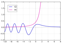
Scorersche Funktionen

Funktionsgraphen von G i ( x ) {\displaystyle \mathrm {Gi} (x)} und H i ( x ) {\displaystyle \mathrm {Hi} (x)} .

Manchmal werden auch die beiden weiteren Funktionen G i ( x ) {\displaystyle \mathrm {Gi} (x)} und H i ( x ) {\displaystyle \mathrm {Hi} (x)} zu den Airy-Funktionen dazugerechnet. Die Integral-Definitionen lauten[4]

G i ( x ) = 1 π 0 sin ( t 3 3 + x t ) d t {\displaystyle \mathrm {Gi} (x)={\frac {1}{\pi }}\int \limits _{0}^{\infty }\sin \left({\frac {t^{3}}{3}}+xt\right)\,\mathrm {d} t}
H i ( x ) = 1 π 0 exp ( t 3 3 + x t ) d t {\displaystyle \mathrm {Hi} (x)={\frac {1}{\pi }}\int \limits _{0}^{\infty }\exp \left(-{\frac {t^{3}}{3}}+xt\right)\,\mathrm {d} t}

Sie lassen sich auch durch die Funktionen A i {\displaystyle \mathrm {Ai} } und B i {\displaystyle \mathrm {Bi} } darstellen.

Literatur

  • Milton Abramowitz, Irene A. Stegun: Handbook of Mathematical Functions with Formulas, Graphs, and Mathematical Tables. (siehe §10.4). National Bureau of Standards, 1954.
  • George Biddell Airy: On the intensity of light in the neighbourhood of a caustic. In: Transactions of the Cambridge Philosophical Society. Band 6, 1838, S. 379–402.
  • Frank Olver: Asymptotics and Special Functions. Chapter 11. Academic Press, New York 1974.
Commons: Airy-Funktion – Sammlung von Bildern, Videos und Audiodateien
  • Eric W. Weisstein: Airy Functions. In: MathWorld (englisch).
  • Bessel-Type Functions. Wolfram Funktionenseite.
  • Chapter 9: Airy and related functions. In: Digital Library of Mathematical Functions.

Einzelnachweise

  1. Eric W. Weisstein: Airy Function Zeros. In: MathWorld (englisch).
  2. C. Banderier, P. Flajolet, G. Schaeffer, M. Soria: Planar Maps and Airy Phenomena. In Automata, Languages and Programming. Proceedings of the 27th International Colloquium (ICALP 2000) held at the University of Geneva, Geneva, 9.–15. Juli 2000 (Ed. U. Montanari, J. D. P. Rolim, E. Welzl). Berlin: Springer, S. 388–402, 2000
  3. Eric W. Weisstein: Airy Zeta Function. In: MathWorld (englisch).
  4. Milton Abramowitz und Irene A. Stegun: Handbook of Mathematical Functions with Formulas, Graphs, and Mathematical Tables, 1954, Seite 447