Reeller projektiver Raum

Ein reeller projektiver Raum ist in der Mathematik der projektive Raum eines reellen Vektorraumes, welcher als Punkte sämtliche reelle Ursprungsgeraden (eindimensionale Untervektorräume) von diesem enthält. R P n {\displaystyle \mathbb {R} P^{n}} notiert dabei den projektiven Raum von R n + 1 {\displaystyle \mathbb {R} ^{n+1}} und wird n {\displaystyle n} -ter reeller projektiver Raum genannt. Ein reeller projektiver Raum ist ein Spezialfall einer Graßmann-Mannigfaltigkeit durch R P n = Gr 1 ( R n + 1 ) {\displaystyle \mathbb {R} P^{n}=\operatorname {Gr} _{1}(\mathbb {R} ^{n+1})} .

Konstruktion

Darstellung der reellen projektiven Ebene, bei der die roten und blauen Seiten entsprechend der durch die Pfeile gegebenen Orientierung miteinander identifiziert werden.

Auf dem reellen euklidischen Raum R n + 1 { 0 } {\displaystyle \mathbb {R} ^{n+1}\setminus \{0\}} ohne Ursprung ist die Relation x y {\displaystyle x\sim y} , wenn es einen reellen Skalar λ R { 0 } {\displaystyle \lambda \in \mathbb {R} \setminus \{0\}} mit x = λ y {\displaystyle x=\lambda y} gibt, eine Äquivalenzrelation. R P n {\displaystyle \mathbb {R} P^{n}} ist der Faktorraum von R n + 1 { 0 } {\displaystyle \mathbb {R} ^{n+1}\setminus \{0\}} unter dieser Äquivalenzrelation.[1] Die Äquivalenzklasse einer Koordinate ( x 0 , , x n ) R n 1 { 0 } {\displaystyle (x_{0},\ldots ,x_{n})\in \mathbb {R} ^{n-1}\setminus \{0\}} wird als [ x 0 : : x n ] R P n {\displaystyle [x_{0}:\ldots :x_{n}]\in \mathbb {R} P^{n}} notiert. Dieser Raum ist eine (reelle) Mannigfaltigkeit, was an der alternativen Definition durch die eindimensionalen Untervektorräume von R n + 1 {\displaystyle \mathbb {R} ^{n+1}} , also als Graßmann-Mannigfaltigkeit R P n = Gr 1 ( R n + 1 ) {\displaystyle \mathbb {R} P^{n}=\operatorname {Gr} _{1}(\mathbb {R} ^{n+1})} , erkennbar ist. Dabei gilt:

dim R R P n = n . {\displaystyle \dim _{\mathbb {R} }\mathbb {R} P^{n}=n.}

Eine alternative Konstruktion ist die Einschränkung auf die Sphären S n R n + 1 { 0 } {\displaystyle S^{n}\subset \mathbb {R} ^{n+1}\setminus \{0\}} und S 0 R { 0 } {\displaystyle S^{0}\subset \mathbb {R} \setminus \{0\}} bei der Betrachtung dieser Äquivalenzrelation.[1] Dadurch ergibt sich ein Faserbündel:[2]

S 0 S n R P n . {\displaystyle S^{0}\rightarrow S^{n}\rightarrow \mathbb {R} P^{n}.}

Da die Faser S 0 Z 2 {\displaystyle S^{0}\cong \mathbb {Z} _{2}} diskret ist, ist die Abbildung S n R P n {\displaystyle S^{n}\rightarrow \mathbb {R} P^{n}} eine doppelte Überlagerung.

Alternative Darstellung der reellen projektiven Ebene

Niedrigdimensionale Beispiele

  • R P 0 {\displaystyle \mathbb {R} P^{0}} ist der einpunktige Raum.
  • R P 1 {\displaystyle \mathbb {R} P^{1}} wird reelle projektive Linie genannt und ist homöomorph zur 1 {\displaystyle 1} -Sphäre S 1 {\displaystyle S^{1}} .[3] Die zusammen mit der kanonischen Projektion R 2 R P 1 {\displaystyle \mathbb {R} ^{2}\rightarrow \mathbb {R} P^{1}} erzeugte Abbildung R 2 S 1 S 1 R P 1 {\displaystyle \mathbb {R} ^{2}\supset S^{1}\rightarrow S^{1}\cong \mathbb {R} P^{1}} zwischen Sphären ist die reele Hopf-Faserung h R {\displaystyle h_{\mathbb {R} }} .[4]
  • R P 2 {\displaystyle \mathbb {R} P^{2}} wird reelle projektive Ebene genannt. Ihre Immersion in R 3 {\displaystyle \mathbb {R} ^{3}} ist bekannt als Boysche Fläche und es gibt eine Einbettung in R 4 {\displaystyle \mathbb {R} ^{4}} . Das Problem von Immersion und Einbettung des reellen projektiven Raumes R P n {\displaystyle \mathbb {R} P^{n}} ist bereits gut untersucht.[5]
  • R P 3 {\displaystyle \mathbb {R} P^{3}} ist diffeomorph zur Drehgruppe SO ( 3 ) {\displaystyle \operatorname {SO} (3)} und besitzt daher eine Gruppenstruktur.[6] Die doppelte Überlagerung S 3 R P 3 {\displaystyle S^{3}\rightarrow \mathbb {R} P^{3}} ist dabei topologisch zugrundeliegend für die doppelte Überlagerung Spin ( 3 ) SO ( 3 ) {\displaystyle \operatorname {Spin} (3)\rightarrow \operatorname {SO} (3)} . (Entsprechend ist S 3 {\displaystyle S^{3}} diffeomorph zur Spingruppe Spin ( 3 ) {\displaystyle \operatorname {Spin} (3)} und besitzt daher ebenfalls eine Gruppenstruktur.)
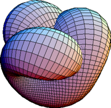
Bryant–Kusner-Parametrisierung der Boyschen Fläche

Eigenschaften

  • Jede stetige Abbildung R P n R P n {\displaystyle \mathbb {R} P^{n}\rightarrow \mathbb {R} P^{n}} mit n {\displaystyle n} gerade hat einen Fixpunkt (also R P n {\displaystyle \mathbb {R} P^{n}} die Fixpunkteigenschaft für n {\displaystyle n} gerade).[7][8] Für n {\displaystyle n} ungerade gilt dies nicht, da dann die Abbildung R P n R P n , [ x 0 : x 1 : . . . . : x n 1 : x n ] [ x 1 : x 0 : . . . . : x n : x n 1 ] {\displaystyle \mathbb {R} P^{n}\rightarrow \mathbb {R} P^{n},[x_{0}:x_{1}:....:x_{n-1}:x_{n}]\mapsto [x_{1}:-x_{0}:....:x_{n}:-x_{n-1}]} keinen Fixpunkt hat.[8]
  • Die reelle projektive Ebene R P 2 {\displaystyle \mathbb {RP} ^{2}} ist der Moore-Raum M ( Z 2 , 1 ) {\displaystyle M(\mathbb {Z} _{2},1)} . Ihre n {\displaystyle n} -fache Einhängung Σ n R P 2 {\displaystyle \Sigma ^{n}\mathbb {R} P^{2}} ist daher der Moore-Raum M ( Z 2 , n + 1 ) {\displaystyle M(\mathbb {Z} _{2},n+1)} .
  • Die kleinste natürliche Zahl k N {\displaystyle k\in \mathbb {N} } , sodass R P n {\displaystyle \mathbb {R} P^{n}} mit n 1 , 3 , 7 {\displaystyle n\neq 1,3,7} eine Einbettung in R k 1 {\displaystyle \mathbb {R} ^{k-1}} besitzt, ist genau die topologische Komplexität TC ( R P n ) {\displaystyle \operatorname {TC} (\mathbb {R} P^{n})} (mit der Konvention TC ( { } ) = 1 {\displaystyle \operatorname {TC} (\{*\})=1} ).[9]
  • Für n = 1 , 3 , 7 {\displaystyle n=1,3,7} ist TC ( R P n ) = n + 1 {\displaystyle \operatorname {TC} (\mathbb {R} P^{n})=n+1} .[9]

CW-Struktur

Der reelle projektive Raum R P n {\displaystyle \mathbb {R} P^{n}} ist ein CW-Komplex. R P n {\displaystyle \mathbb {R} P^{n}} entsteht aus R P n 1 {\displaystyle \mathbb {R} P^{n-1}} durch Anklebung einer n {\displaystyle n} -Zelle. Da R P 0 {\displaystyle \mathbb {R} P^{0}} aus einer 0 {\displaystyle 0} -Zelle besteht, hat die CW-Struktur auf R P n {\displaystyle \mathbb {R} P^{n}} daher eine Zelle in jeder Dimension k {\displaystyle k} von 0 k n {\displaystyle 0\leq k\leq n} .[10][11]

Algebraische Topologie

Homotopie

Die Homotopiegruppen des reellen projektiven Raumes R P n {\displaystyle \mathbb {R} P^{n}} lassen sich über die lange exakte Sequenz von Homotopiegruppen[12] des Faserbündels S 0 S n R P n {\displaystyle S^{0}\rightarrow S^{n}\rightarrow \mathbb {R} P^{n}} berechnen[13] und sind gegeben durch:[14]

π k ( R P n ) = { 0 ; k = 0 Z ; k = 1 , n = 1 Z 2 ; k = 1 , n > 1 π k ( S n ) ; k > 1 , n > 0 . {\displaystyle \pi _{k}(\mathbb {R} P^{n})={\begin{cases}0&;k=0\\\mathbb {Z} &;k=1,n=1\\\mathbb {Z} _{2}&;k=1,n>1\\\pi _{k}(S^{n})&;k>1,n>0\end{cases}}.}

Homologie

Die Homologiegruppen des reellen projektiven Raumes R P n {\displaystyle \mathbb {R} P^{n}} lassen sich über zelluläre Homologie aus dessen CW-Struktur berechnen und sind gegeben durch:[15][16]

H k ( R P n ) { Z ; k = 0  oder  k = n  wenn ungerade Z 2 ; k  ungerade , 0 < k < n 1 ; sonst. . {\displaystyle H_{k}(\mathbb {R} P^{n})\cong {\begin{cases}\mathbb {Z} &;k=0{\text{ oder }}k=n{\text{ wenn ungerade}}\\\mathbb {Z} _{2}&;k{\text{ ungerade}},0<k<n\\1&;{\text{sonst.}}\end{cases}}.}

Es ist also H n 1 ( R P n ) Z 2 {\displaystyle H_{n-1}(\mathbb {R} P^{n})\cong \mathbb {Z} _{2}} für n {\displaystyle n} gerade und H n 1 ( R P n ) 1 {\displaystyle H_{n-1}(\mathbb {R} P^{n})\cong 1} für n {\displaystyle n} ungerade. Daraus folgt,[17] dass R P n {\displaystyle \mathbb {R} P^{n}} genau dann orientierbar ist, wenn n {\displaystyle n} ungerade ist.[18]

Kohomologie

Die Kohomologiegruppen des reellen projektiven Raumes R P n {\displaystyle \mathbb {R} P^{n}} sind gegeben durch:[19]

H k ( R P n ) { Z ; k = 0  oder  k = n  wenn ungerade Z 2 ; k  ungerade , 0 < k < n 1 ; sonst. . {\displaystyle H^{k}(\mathbb {R} P^{n})\cong {\begin{cases}\mathbb {Z} &;k=0{\text{ oder }}k=n{\text{ wenn ungerade}}\\\mathbb {Z} _{2}&;k{\text{ ungerade}},0<k<n\\1&;{\text{sonst.}}\end{cases}}.}

Für den Kohomologiering gilt:[20]

H ( R P n ; Z 2 ) = Z 2 [ w 1 ] / ( w 1 n + 1 ) , {\displaystyle H^{*}(\mathbb {R} P^{n};\mathbb {Z} _{2})=\mathbb {Z} _{2}[w_{1}]/(w_{1}^{n+1}),}

wobei w 1 {\displaystyle w_{1}} die erste Stiefel–Whitney-Klasse ist.

K-Theorie

Tautologisches Linienbündel

Es gibt ein kanonisches Linienbündel über dem reellen projektiven Raum R P n {\displaystyle \mathbb {R} P^{n}} , da dessen Punkte per Konstruktion aus eindimensionalen Untervektorräumen bestehen, definiert durch:

γ R 1 , n := { ( x , V ) R n + 1 × R P n | x V } {\displaystyle \gamma _{\mathbb {R} }^{1,n}:=\{(x,V)\in \mathbb {R} ^{n+1}\times \mathbb {R} P^{n}|x\in V\}}
π R 1 , n : γ R 1 , n R P n , ( x , V ) V . {\displaystyle \pi _{\mathbb {R} }^{1,n}\colon \gamma _{\mathbb {R} }^{1,n}\rightarrow \mathbb {R} P^{n},(x,V)\mapsto V.}

Das ist ein Spezialfall des tautologischen Vektorbündels über Graßmann-Mannigfaltigkeiten.[21]

Tangentialbündel

Für das Tangentialbündel des reellen projektiven Raumes R P n {\displaystyle \mathbb {R} P^{n}} gilt:[22]

T R P n R _ ( γ R 1 , n ) n + 1 . {\displaystyle T\mathbb {R} P^{n}\oplus {\underline {\mathbb {R} }}\cong (\gamma _{\mathbb {R} }^{1,n})^{n+1}.}

Unendlicher reeller projektiver Raum

Die kanonische Inklusion R n + 1 R n + 2 , x ( x , 0 ) {\displaystyle \mathbb {R} ^{n+1}\hookrightarrow \mathbb {R} ^{n+2},x\mapsto (x,0)} erzeugt eine wohldefinierte kanonische Inklusion R P n R P n + 1 , [ x ] [ ( x , 0 ) ] {\displaystyle \mathbb {R} P^{n}\hookrightarrow \mathbb {R} P^{n+1},[x]\mapsto [(x,0)]} . Der direkte Limes dieser Kette an Inklusionen wird als:

R P := lim n R P n {\displaystyle \mathbb {R} P^{\infty }:=\lim _{n\rightarrow \infty }\mathbb {R} P^{n}}

bezeichnet und unendlicher reeller projektiver Raum genannt.[23]

Das obige Faserbündel S 0 S n R P n {\displaystyle S^{0}\rightarrow S^{n}\rightarrow \mathbb {R} P^{n}} erzeugt durch direkten Limes ein Faserbündel S 0 S R P {\displaystyle S^{0}\rightarrow S^{\infty }\rightarrow \mathbb {R} P^{\infty }} . Da die unendlich-dimensionale Sphäre S {\displaystyle S^{\infty }} zusammenziehbar ist (also alle Homotopiegruppen verschwinden),[24] folgt aus der langen exakten Sequenz von Homotopiegruppen[12] für die des unendlich reellen projektiven Raumes R P {\displaystyle \mathbb {R} P^{\infty }} :

π k ( R P ) π k 1 ( S 0 ) = { Z 2 ; k = 1 1 ; sonst. . {\displaystyle \pi _{k}(\mathbb {R} P^{\infty })\cong \pi _{k-1}(S^{0})={\begin{cases}\mathbb {Z} _{2}&;k=1\\1&;{\text{sonst.}}\end{cases}}.}

Die CW-Struktur überträgt sich ebenfalls durch den direkten Limes, sodass der unendliche reelle projektive Raum R P {\displaystyle \mathbb {R} P^{\infty }} eine CW-Struktur mit einer Zelle in jeder Dimension hat.

Das tautologische Linienbündel lässt sich durch den direkten Limes γ R 1 := lim n γ R 1 , n {\displaystyle \gamma _{\mathbb {R} }^{1}:=\lim _{n\rightarrow \infty }\gamma _{\mathbb {R} }^{1,n}} über die kanonischen Inklusionen γ R 1 , n γ R 1 , n + 1 , ( x , V ) ( ( x , 0 ) , V × { 0 } ) {\displaystyle \gamma _{\mathbb {R} }^{1,n}\hookrightarrow \gamma _{\mathbb {R} }^{1,n+1},(x,V)\mapsto ((x,0),V\times \{0\})} auf R P {\displaystyle \mathbb {R} P^{\infty }} fortsetzen und ist ein Spezialfall eines universellen Vektorbündels. Die Namensgebung kommt daher, dass sich jedes reelle Linienbündel als zurückgezogenes Vektorbündel aus diesem erhalten lässt, also für jedes reelle Linienbündel π : E B {\displaystyle \pi \colon E\rightarrow B} mit B {\displaystyle B} parakompakt (bis auf Homotopie) eine klassifizierende Abbildung f : B R P {\displaystyle f\colon B\rightarrow \mathbb {R} P^{\infty }} existiert, sodass π = f π R 1 {\displaystyle \pi =f^{*}\pi _{\mathbb {R} }^{1}} . Es gibt daher eine Isomorphie von Mengen:[25]

Vect R 1 ( B ) [ B , R P ] . {\displaystyle \operatorname {Vect} _{\mathbb {R} }^{1}(B)\cong [B,\mathbb {R} P^{\infty }].}

Etwa ist der Rückzug des universellen Vektorbündels γ R 1 {\displaystyle \gamma _{\mathbb {R} }^{1}} entlang der kanonischen Inklusion R P n R P {\displaystyle \mathbb {R} P^{n}\hookrightarrow \mathbb {R} P^{\infty }} (also B = R P n {\displaystyle B=\mathbb {R} P^{n}} ) wieder das tautologische Linienbündel γ R 1 , n {\displaystyle \gamma _{\mathbb {R} }^{1,n}} .

R P {\displaystyle \mathbb {R} P^{\infty }} ist BO ( 1 ) {\displaystyle \operatorname {BO} (1)} , der klassifizierende Raum von O ( 1 ) {\displaystyle \operatorname {O} (1)} , der ersten orthogonalen Gruppe, und dadurch ebenso K ( Z 2 , 1 ) {\displaystyle K(\mathbb {Z} _{2},1)} ,[26][23] der erste Eilenberg–MacLane-Raum von π 0 O ( 1 ) Z 2 {\displaystyle \pi _{0}\operatorname {O} (1)\cong \mathbb {Z} _{2}} wie oben bereits gezeigt. Das bedeutet, dass R P {\displaystyle \mathbb {R} P^{\infty }} die erste singuläre Kohomologie mit Koeffizienten in Z 2 {\displaystyle \mathbb {Z} _{2}} darstellt (vergleiche mit dem Brownschen Darstellungssatz), also für topologische Räume B {\displaystyle B} mit dem Homotopietyp eines CW-Komplexes (also insbesondere parakompakt[27]) sogar spezieller gilt:

Vect R 1 ( B ) [ B , R P ] H 1 ( B ; Z 2 ) . {\displaystyle \operatorname {Vect} _{\mathbb {R} }^{1}(B)\cong [B,\mathbb {R} P^{\infty }]\cong H^{1}(B;\mathbb {Z} _{2}).}

Dabei ist der Isomorphismus (Homomorphismus, falls B {\displaystyle B} nicht vom Homotopietyp eines CW-Komplexes ist) durch die erste Stiefel–Whitney-Klasse w 1 : Vect R 1 ( B ) H 1 ( B ; Z 2 ) {\displaystyle w_{1}\colon \operatorname {Vect} _{\mathbb {R} }^{1}(B)\rightarrow H^{1}(B;\mathbb {Z} _{2})} gegeben.[28]

Der Kohomologiering des unendlich reellen projektiven Raumes R P {\displaystyle \mathbb {R} P^{\infty }} mit Koeffizienten in Z 2 {\displaystyle \mathbb {Z} _{2}} ist gegeben durch:[20]

H ( R P ; Z 2 ) = Z 2 [ w 1 ] , {\displaystyle H^{*}(\mathbb {R} P^{\infty };\mathbb {Z} _{2})=\mathbb {Z} _{2}[w_{1}],}

wobei w 1 {\displaystyle w_{1}} die erste Stiefel–Whitney-Klasse ist. Das folgt direkt aus dem allgemeineren Resultat für den klassifizierenden Raum von O ( n ) {\displaystyle \operatorname {O} (n)} :[29][30]

H ( BO ( n ) ; Z 2 ) = Z 2 [ w 1 , , w n ] . {\displaystyle H^{*}(\operatorname {BO} (n);\mathbb {Z} _{2})=\mathbb {Z} _{2}[w_{1},\ldots ,w_{n}].}

Siehe auch

Literatur

  • Allen Hatcher: Algebraic Topology. Cambridge University Press, 2001, ISBN 978-0-521-79160-1 (englisch, cornell.edu). 
  • Allen Hatcher: Vector Bundles and K-Theory. (englisch, cornell.edu [PDF]). 
  • Glen Bredon: Topology and geometry,. Hrsg.: Graduate Texts in Mathematics. Springer Verlag, 1993 (englisch). 
  • Donald Davis: Table of immersions and embeddings of real projective spaces. Abgerufen am 22. September 2011 (englisch). 

Weblinks

Einzelnachweise

  1. a b Allen Hatcher: Algebraic Topology. S. 6, Example 0.4. 
  2. Allen Hatcher: Algebraic Topology. S. 377, Example 4.44. (englisch). 
  3. projective space. Abgerufen am 31. Januar 2024 (englisch). 
  4. real Hopf fibration. Abgerufen am 31. Januar 2024 (englisch). 
  5. Siehe Don Davis für ein Literaturverzeichnis und eine Liste an bekannten Resultaten.
  6. Allen Hatcher: Algebraic Topology. S. 293. 
  7. Allen Hatcher: Algebraic Topology. S. 155, Exercise 2. 
  8. a b Allen Hatcher: Algebraic Topology. S. 180. 
  9. a b Michael Farber, Serge Tabachnikov, Sergey Yuzvinsky: Topological robotics: motion planning in projective spaces. 2. Oktober 2002, abgerufen am 31. Januar 2024 (englisch). 
  10. cell structure of projective spaces. Abgerufen am 31. Januar 2024 (englisch). 
  11. CW structure of real projective space. Abgerufen am 31. Januar 2024 (englisch). 
  12. a b Allen Hatcher: Algebraic Topology. S. 376, Theorem 4.41. 
  13. Allen Hatcher: Algebraic Topology. S. 380, Example 4.49. 
  14. Homotopy of real projective space. Abgerufen am 31. Januar 2024 (englisch). 
  15. Hatcher: Algebraic Topology. Chapter 2: Homology, Example 2.42, S. 144 (englisch). 
  16. Homology of real projective space. Abgerufen am 30. Januar 2024 (englisch). 
  17. Allen Hatcher: Algebraic Topology. S. 238, Corollary 3.28. 
  18. J. T. Wloka, B. Rowley, B. Lawruk: Boundary Value Problems for Elliptic Systems. Cambridge University Press, 1995, ISBN 978-0-521-43011-1, S. 197 (englisch, google.com). 
  19. Cohomology of real projective space. Abgerufen am 30. Januar 2024 (englisch). 
  20. a b Allen Hatcher: Algebraic Topology. S. 213/220, Example 3.12/Theorem 3.19. 
  21. Allen Hatcher: Vector Bundles and K-theory. S. 6–7. 
  22. Allen Hatcher: Vector Bundles and K-theory. S. 11. 
  23. a b real projective space. Abgerufen am 31. Januar 2024 (englisch). 
  24. Allen Hatcher: Algebraic Topology. S. 19, Exercise 16. 
  25. Allen Hatcher: Vector Bundles and K-theory. S. 29, Theorem 1.16. 
  26. Allen Hatcher: Algebraic Topology. S. 88, Example 1B.3. 
  27. Allen Hatcher: Algebraic Topology. S. 36, Proposition 1.20. 
  28. Allen Hatcher: Vector Bundles and K-theory. S. 86, Proposition 3.10. 
  29. John Milnor, James Stasheff: Characteristic Classes. S. 83, Theorem 7.1. 
  30. Stiefel-Whitney class. Abgerufen am 18. Februar 2024 (englisch).