Taburan normal

Taburan normal

Keluk merah ialah taburan normal piawai
Fungsi pengedaran kumulatif
Tatatanda	${\displaystyle {\mathcal {N}}(\mu ,\sigma ^{2})}$
Parameter	${\displaystyle \mu \in \mathbb {R} }$ = min (lokasi) ${\displaystyle \sigma ^{2}\in \mathbb {R} _{>0}}$ = varians (skala kuasa dua)
Sokongan	${\displaystyle x\in \mathbb {R} }$
PDF	${\displaystyle {\frac {1}{\sigma {\sqrt {2\pi }}}}e^{-{\frac {1}{2}}\left({\frac {x-\mu }{\sigma }}\right)^{2}}}$
CDF	${\displaystyle {\frac {1}{2}}\left[1+\operatorname {erf} \left({\frac {x-\mu }{\sigma {\sqrt {2}}}}\right)\right]}$
Kuantil	${\displaystyle \mu +\sigma {\sqrt {2}}\operatorname {erf} ^{-1}(2p-1)}$
Min	${\displaystyle \mu }$
Median	${\displaystyle \mu }$
Mod	${\displaystyle \mu }$
Varians	${\displaystyle \sigma ^{2}}$
MAD	${\displaystyle \sigma {\sqrt {2/\pi }}}$
Kecondongan	${\displaystyle 0}$
Ex. kurtosis	${\displaystyle 0}$
Entropi	${\displaystyle {\frac {1}{2}}\log(2\pi \sigma ^{2})+{\frac {1}{2}}}$
MGF	${\displaystyle \exp(\mu t+\sigma ^{2}t^{2}/2)}$
CF	${\displaystyle \exp(i\mu t-\sigma ^{2}t^{2}/2)}$
Maklumat Fisher	${\displaystyle {\mathcal {I}}(\mu ,\sigma )={\begin{pmatrix}1/\sigma ^{2}&0\\0&2/\sigma ^{2}\end{pmatrix}}}$ ${\displaystyle {\mathcal {I}}(\mu ,\sigma ^{2})={\begin{pmatrix}1/\sigma ^{2}&0\\0&1/(2\sigma ^{4})\end{pmatrix}}}$
Perbezaan Kullback-Leibler	${\displaystyle {1 \over 2}\left\{\left({\frac {\sigma _{0}}{\sigma _{1}}}\right)^{2}+{\frac {(\mu _{1}-\mu _{0})^{2}}{\sigma _{1}^{2}}}-1+2\ln {\sigma _{1} \over \sigma _{0}}\right\}}$

Sebahagian daripada siri tentang statistik
Teori kebarangkalian
Kebarangkalian Aksiom Determinisme Sistem Indeterminisme Rawak
Ruang kebarangkalian Ruang sampel Peristiwa Peristiwa menyeluruh secara kolektif Peristiwa asas Keeksklusifan bersama Hasil Singleton Eksperimen Percubaan Bernoulli Taburan kebarangkalian Taburan Bernoulli Taburan binomial Taburan normal Ukuran kebarangkalian Pemboleh ubah rawak Proses Bernoulli Selanjar atau diskret Nilai jangkaan Rantaian Markov Nilai diperhatikan Jalan rawak Proses stokastik
Peristiwa pelengkap Kebarangkalian bersama Kebarangkalian marginal Kebarangkalian bersyarat
Kebebasan Kebebasan bersyarat Hukum jumlah kebarangkalian Hukum nombor besar Teorem Bayes Ketaksamaan Boole
Gambar rajah Venn Gambar rajah pokok
l b s

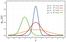
Dalam teori kebarangkalian, taburan normal (juga dikenali sebagai taburan Gaussian, Gauss, atau Laplace–Gauss) ialah sejenis taburan kebarangkalian selanjar untuk pemboleh ubah rawak bernilai nyata. Bentuk umum fungsi ketumpatan kebarangkaliannya ialah

${\displaystyle f(x)={\frac {1}{\sigma {\sqrt {2\pi }}}}e^{-{\frac {1}{2}}\left({\frac {x-\mu }{\sigma }}\right)^{2}}}$

Parameter ${\displaystyle \mu }$ ialah min atau jangkaan taburan (dan juga median dan mod), manakala parameter ${\displaystyle \sigma }$ ialah sisihan piawai. Varians taburan ini ialah ${\displaystyle \sigma ^{2}}$.^[1] Pemboleh ubah rawak dengan taburan Gaussian dikatakan sebagai ditaburkan secara normal, dan dipanggil simpangan normal.

Taburan normal adalah penting dalam statistik dan sering digunakan dalam sains semula jadi dan sosial untuk mewakili pemboleh ubah rawak bernilai-nyata yang taburannya tidak diketahui.^[2][3] Kepentingan mereka sebahagiannya disebabkan oleh teorem had pusat. Ia menyatakan bahawa, di bawah beberapa keadaan, purata banyak sampel (pemerhatian) pemboleh ubah rawak dengan min dan varians terhingga itu sendiri adalah pemboleh ubah rawak—yang taburannya menumpu kepada taburan normal ketika bilangan sampel bertambah. Oleh itu, kuantiti fizik yang dijangka menjadi jumlah banyak proses bebas, seperti ralat pengukuran, selalunya mempunyai taburan yang hampir normal.^[4]

Selain itu, taburan Gaussian mempunyai beberapa sifat unik yang bernilai dalam kajian analitik. Sebagai contoh, sebarang kombinasi linear bagi koleksi tetap sisihan normal ialah sisihan normal. Banyak keputusan dan kaedah, seperti penyesuaian parameter penyebaran ketidakpastian dan kuasa dua terkecil, boleh diterbitkan secara analitikal dalam bentuk eksplisit apabila pemboleh ubah yang berkaitan ditabur secara normal.

Taburan normal kadangkala dipanggil lengkung loceng secara tidak rasmi.^[5] Walau bagaimanapun, banyak taburan lain juga berbentuk loceng (seperti taburan Cauchy, t Pelajar dan logistik).

Taburan kebarangkalian univariat digeneralisasikan untuk vektor dalam taburan normal multivariat dan untuk matriks dalam taburan normal matriks.

Definisi

Taburan normal piawai

Kes paling mudah bagi taburan normal dikenali sebagai taburan normal piawai atau taburan normal unit. Ini adalah kes istimewa apabila ${\displaystyle \mu =0}$ dan ${\displaystyle \sigma =1}$, dan ia diterangkan oleh fungsi ketumpatan kebarangkalian (atau ketumpatan) ini:

${\displaystyle \varphi (z)={\frac {e^{-{\frac {z^{2}}{2}}}}{\sqrt {2\pi }}}}$

Pemboleh ubah ${\displaystyle z}$ mempunyai min 0 dan varians dan sisihan piawai 1. Ketumpatan ${\displaystyle \varphi (z)}$ mempunyai kemuncaknya ${\displaystyle 1/{\sqrt {2\pi }}}$ di ${\displaystyle z=0}$ dan titik lengkok balas pada ${\displaystyle z=+1}$ dan ${\displaystyle z=-1}$.

Walaupun ketumpatan di atas paling biasa dikenali sebagai normal piawai (bahasa Inggeris: standard normal), beberapa pengarang telah menggunakan istilah itu untuk menerangkan versi lain bagi taburan normal. Carl Friedrich Gauss, sebagai contoh, sekali mentakrifkan normal piawai sebagai

${\displaystyle \varphi (z)={\frac {e^{-z^{2}}}{\sqrt {\pi }}}}$

yang mempunyai varians 1/2, dan Stephen Stigler^[6] pernah mentakrifkan normal piawai sebagai

${\displaystyle \varphi (x)=e^{-\pi z^{2}}}$

yang mempunyai bentuk fungsian mudah dan varians ${\displaystyle \sigma ^{2}=1/(2\pi )}$:

Rujukan

Petikan

Sumber

Pautan luar

• Hazewinkel, Michiel, penyunting (2001), "Normal distribution", Encyclopedia of Mathematics, Springer, ISBN 978-1-55608-010-4
• Kalkulator taburan normal, Kalkulator yang lebih berkuasa