Kaniadakis Gaussian distribution

κ-Gaussian distribution

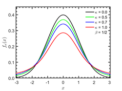
Probability density function
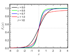
Cumulative distribution function
Parameters	${\displaystyle 0<\kappa <1}$ shape (real) ${\displaystyle \beta >0}$ rate (real)
Support	${\displaystyle x\in \mathbb {R} }$
PDF	${\displaystyle Z_{\kappa }\exp _{\kappa }(-\beta x^{2})\,\,\,;\,\,\,Z_{\kappa }={\sqrt {\frac {2\beta \kappa }{\pi }}}{\Bigg (}1+{\frac {1}{2}}\kappa {\Bigg )}{\frac {\Gamma {\Big (}{\frac {1}{2\kappa }}+{\frac {1}{4}}{\Big )}}{\Gamma {\Big (}{\frac {1}{2\kappa }}-{\frac {1}{4}}{\Big )}}}}$
CDF	${\displaystyle {\frac {1}{2}}+{\frac {1}{2}}{\textrm {erf}}_{\kappa }{\big (}{\sqrt {\beta }}x{\big )}\ }$
Mean	${\displaystyle 0}$
Median	${\displaystyle 0}$
Mode	${\displaystyle 0}$
Variance	${\displaystyle \sigma _{\kappa }^{2}={\frac {1}{\beta }}{\frac {2+\kappa }{2-\kappa }}{\frac {4\kappa }{4-9\kappa ^{2}}}\left[{\frac {\Gamma {\Big (}{\frac {1}{2\kappa }}+{\frac {1}{4}}{\Big )}}{\Gamma {\Big (}{\frac {1}{2\kappa }}-{\frac {1}{4}}{\Big )}}}\right]^{2}}$
Skewness	${\displaystyle 0}$
Excess kurtosis	${\displaystyle 3\left[{\frac {{\sqrt {\pi }}Z_{\kappa }}{2\beta ^{2/3}\sigma _{\kappa }^{4}}}{\frac {(2\kappa )^{-5/2}}{1+{\frac {5}{2}}\kappa }}{\frac {\Gamma \left({\frac {1}{2\kappa }}-{\frac {5}{4}}\right)}{\Gamma \left({\frac {1}{2\kappa }}+{\frac {5}{4}}\right)}}-1\right]}$

The Kaniadakis Gaussian distribution (also known as κ-Gaussian distribution) is a probability distribution which arises as a generalization of the Gaussian distribution from the maximization of the Kaniadakis entropy under appropriated constraints. It is one example of a Kaniadakis κ-distribution. The κ-Gaussian distribution has been applied successfully for describing several complex systems in economy,^[1] geophysics,^[2] astrophysics, among many others.

The κ-Gaussian distribution is a particular case of the κ-Generalized Gamma distribution.^[3]

Definitions

Probability density function

The general form of the centered Kaniadakis κ-Gaussian probability density function is:^[3]

${\displaystyle f_{_{\kappa }}(x)=Z_{\kappa }\exp _{\kappa }(-\beta x^{2})}$

where ${\displaystyle |\kappa |<1}$ is the entropic index associated with the Kaniadakis entropy, ${\displaystyle \beta >0}$ is the scale parameter, and

${\displaystyle Z_{\kappa }={\sqrt {\frac {2\beta \kappa }{\pi }}}{\Bigg (}1+{\frac {1}{2}}\kappa {\Bigg )}{\frac {\Gamma {\Big (}{\frac {1}{2\kappa }}+{\frac {1}{4}}{\Big )}}{\Gamma {\Big (}{\frac {1}{2\kappa }}-{\frac {1}{4}}{\Big )}}}}$

is the normalization constant.

The standard Normal distribution is recovered in the limit ${\displaystyle \kappa \rightarrow 0.}$

Cumulative distribution function

The cumulative distribution function of κ-Gaussian distribution is given by

${\displaystyle F_{\kappa }(x)={\frac {1}{2}}+{\frac {1}{2}}{\textrm {erf}}_{\kappa }{\big (}{\sqrt {\beta }}x{\big )}}$

where

${\displaystyle {\textrm {erf}}_{\kappa }(x)={\Big (}2+\kappa {\Big )}{\sqrt {\frac {2\kappa }{\pi }}}{\frac {\Gamma {\Big (}{\frac {1}{2\kappa }}+{\frac {1}{4}}{\Big )}}{\Gamma {\Big (}{\frac {1}{2\kappa }}-{\frac {1}{4}}{\Big )}}}\int _{0}^{x}\exp _{\kappa }(-t^{2})dt}$

is the Kaniadakis κ-Error function, which is a generalization of the ordinary Error function ${\displaystyle {\textrm {erf}}(x)}$ as ${\displaystyle \kappa \rightarrow 0}$.

Properties

Moments, mean and variance

The centered κ-Gaussian distribution has a moment of odd order equal to zero, including the mean.

The variance is finite for ${\displaystyle \kappa <2/3}$ and is given by:

${\displaystyle \operatorname {Var} [X]=\sigma _{\kappa }^{2}={\frac {1}{\beta }}{\frac {2+\kappa }{2-\kappa }}{\frac {4\kappa }{4-9\kappa ^{2}}}\left[{\frac {\Gamma \left({\frac {1}{2\kappa }}+{\frac {1}{4}}\right)}{\Gamma \left({\frac {1}{2\kappa }}-{\frac {1}{4}}\right)}}\right]^{2}}$

Kurtosis

The kurtosis of the centered κ-Gaussian distribution may be computed thought:

${\displaystyle \operatorname {Kurt} [X]=\operatorname {E} \left[{\frac {X^{4}}{\sigma _{\kappa }^{4}}}\right]}$

which can be written as

${\displaystyle \operatorname {Kurt} [X]={\frac {2Z_{\kappa }}{\sigma _{\kappa }^{4}}}\int _{0}^{\infty }x^{4}\,\exp _{\kappa }\left(-\beta x^{2}\right)dx}$

Thus, the kurtosis of the centered κ-Gaussian distribution is given by:

${\displaystyle \operatorname {Kurt} [X]={\frac {3{\sqrt {\pi }}Z_{\kappa }}{2\beta ^{2/3}\sigma _{\kappa }^{4}}}{\frac {|2\kappa |^{-5/2}}{1+{\frac {5}{2}}|\kappa |}}{\frac {\Gamma \left({\frac {1}{|2\kappa |}}-{\frac {5}{4}}\right)}{\Gamma \left({\frac {1}{|2\kappa |}}+{\frac {5}{4}}\right)}}}$

or

${\displaystyle \operatorname {Kurt} [X]={\frac {3\beta ^{11/6}{\sqrt {2\kappa }}}{2}}{\frac {|2\kappa |^{-5/2}}{1+{\frac {5}{2}}|\kappa |}}{\Bigg (}1+{\frac {1}{2}}\kappa {\Bigg )}\left({\frac {2-\kappa }{2+\kappa }}\right)^{2}\left({\frac {4-9\kappa ^{2}}{4\kappa }}\right)^{2}\left[{\frac {\Gamma {\Big (}{\frac {1}{2\kappa }}-{\frac {1}{4}}{\Big )}}{\Gamma {\Big (}{\frac {1}{2\kappa }}+{\frac {1}{4}}{\Big )}}}\right]^{3}{\frac {\Gamma \left({\frac {1}{|2\kappa |}}-{\frac {5}{4}}\right)}{\Gamma \left({\frac {1}{|2\kappa |}}+{\frac {5}{4}}\right)}}}$

κ-Error function

κ-Error function
Plot of the κ-error function for typical κ-values. The case κ=0 corresponds to the ordinary error function.
General information
General definition	${\displaystyle \operatorname {erf} _{\kappa }(x)={\Big (}2+\kappa {\Big )}{\sqrt {\frac {2\kappa }{\pi }}}{\frac {\Gamma {\Big (}{\frac {1}{2\kappa }}+{\frac {1}{4}}{\Big )}}{\Gamma {\Big (}{\frac {1}{2\kappa }}-{\frac {1}{4}}{\Big )}}}\int _{0}^{x}\exp _{\kappa }(-t^{2})dt}$
Fields of application	Probability, thermodynamics
Domain, codomain and image
Domain	${\displaystyle \mathbb {C} }$
Image	${\displaystyle \left(-1,1\right)}$
Specific features
Root	${\displaystyle 0}$
Derivative	${\displaystyle {\frac {d}{dx}}\operatorname {erf} _{\kappa }(x)=\left(2+\kappa \right){\sqrt {\frac {2\kappa }{\pi }}}{\frac {\Gamma \left({\frac {1}{2\kappa }}+{\frac {1}{4}}\right)}{\Gamma \left({\frac {1}{2\kappa }}-{\frac {1}{4}}\right)}}\exp _{\kappa }(-x^{2})}$

The Kaniadakis κ-Error function (or κ-Error function) is a one-parameter generalization of the ordinary error function defined as:^[3]

${\displaystyle \operatorname {erf} _{\kappa }(x)={\Big (}2+\kappa {\Big )}{\sqrt {\frac {2\kappa }{\pi }}}{\frac {\Gamma {\Big (}{\frac {1}{2\kappa }}+{\frac {1}{4}}{\Big )}}{\Gamma {\Big (}{\frac {1}{2\kappa }}-{\frac {1}{4}}{\Big )}}}\int _{0}^{x}\exp _{\kappa }(-t^{2})dt}$

Although the error function cannot be expressed in terms of elementary functions, numerical approximations are commonly employed.

For a random variable X distributed according to a κ-Gaussian distribution with mean 0 and standard deviation ${\displaystyle {\sqrt {\beta }}}$, κ-Error function means the probability that X falls in the interval ${\displaystyle [-x,\,x]}$.

Applications

The κ-Gaussian distribution has been applied in several areas, such as:

• In economy, the κ-Gaussian distribution has been applied in the analysis of financial models, accurately representing the dynamics of the processes of extreme changes in stock prices.^[4]
• In inverse problems, Error laws in extreme statistics are robustly represented by κ-Gaussian distributions.^[2][5][6]
• In astrophysics, stellar-residual-radial-velocity data have a Gaussian-type statistical distribution, in which the K index presents a strong relationship with the stellar-cluster ages.^[7][8]
• In nuclear physics, the study of Doppler broadening function in nuclear reactors is well described by a κ-Gaussian distribution for analyzing the neutron-nuclei interaction.^[9][10]
• In cosmology, for interpreting the dynamical evolution of the Friedmann–Robertson–Walker Universe.
• In plasmas physics, for analyzing the electron distribution in electron-acoustic double-layers^[11] and the dispersion of Langmuir waves.^[12]

See also

• Giorgio Kaniadakis
• Kaniadakis statistics
• Kaniadakis distribution
• Kaniadakis κ-Exponential distribution
• Kaniadakis κ-Gamma distribution
• Kaniadakis κ-Weibull distribution
• Kaniadakis κ-Logistic distribution
• Kaniadakis κ-Erlang distribution

References

External links

• Kaniadakis Statistics on arXiv.org

References

[edit]- ^ Moretto, Enrico; Pasquali, Sara; Trivellato, Barbara (2017). "A non-Gaussian option pricing model based on Kaniadakis exponential deformation". The European Physical Journal B. 90 (10): 179. Bibcode:2017EPJB...90..179M. doi:10.1140/epjb/e2017-80112-x. ISSN 1434-6028. S2CID 254116243.
- ^ a b da Silva, Sérgio Luiz E. F.; Carvalho, Pedro Tiago C.; de Araújo, João M.; Corso, Gilberto (2020-05-27). "Full-waveform inversion based on Kaniadakis statistics". Physical Review E. 101 (5): 053311. Bibcode:2020PhRvE.101e3311D. doi:10.1103/PhysRevE.101.053311. ISSN 2470-0045. PMID 32575242. S2CID 219746493.
- ^ a b c Kaniadakis, G. (2021-01-01). "New power-law tailed distributions emerging in κ-statistics (a)". Europhysics Letters. 133 (1): 10002. arXiv:2203.01743. Bibcode:2021EL....13310002K. doi:10.1209/0295-5075/133/10002. ISSN 0295-5075. S2CID 234144356.
- ^ Moretto, Enrico; Pasquali, Sara; Trivellato, Barbara (2017). "A non-Gaussian option pricing model based on Kaniadakis exponential deformation". The European Physical Journal B. 90 (10): 179. Bibcode:2017EPJB...90..179M. doi:10.1140/epjb/e2017-80112-x. ISSN 1434-6028. S2CID 254116243.
- ^ Wada, Tatsuaki; Suyari, Hiroki (2006). "κ-generalization of Gauss' law of error". Physics Letters A. 348 (3–6): 89–93. arXiv:cond-mat/0505313. Bibcode:2006PhLA..348...89W. doi:10.1016/j.physleta.2005.08.086. S2CID 119003351.
- ^ da Silva, Sérgio Luiz E.F.; Silva, R.; dos Santos Lima, Gustavo Z.; de Araújo, João M.; Corso, Gilberto (2022). "An outlier-resistant κ -generalized approach for robust physical parameter estimation". Physica A: Statistical Mechanics and Its Applications. 600: 127554. arXiv:2111.09921. Bibcode:2022PhyA..60027554D. doi:10.1016/j.physa.2022.127554. S2CID 248803855.
- ^ Carvalho, J. C.; Silva, R.; do Nascimento jr., J. D.; Soares, B. B.; De Medeiros, J. R. (2010-09-01). "Observational measurement of open stellar clusters: A test of Kaniadakis and Tsallis statistics". EPL (Europhysics Letters). 91 (6): 69002. Bibcode:2010EL.....9169002C. doi:10.1209/0295-5075/91/69002. ISSN 0295-5075. S2CID 120902898.
- ^ Carvalho, J. C.; Silva, R.; do Nascimento jr., J. D.; De Medeiros, J. R. (2008). "Power law statistics and stellar rotational velocities in the Pleiades". EPL (Europhysics Letters). 84 (5): 59001. arXiv:0903.0836. Bibcode:2008EL.....8459001C. doi:10.1209/0295-5075/84/59001. ISSN 0295-5075. S2CID 7123391.
- ^ Guedes, Guilherme; Gonçalves, Alessandro C.; Palma, Daniel A.P. (2017). "The Doppler Broadening Function using the Kaniadakis distribution". Annals of Nuclear Energy. 110: 453–458. doi:10.1016/j.anucene.2017.06.057.
- ^ de Abreu, Willian V.; Gonçalves, Alessandro C.; Martinez, Aquilino S. (2019). "Analytical solution for the Doppler broadening function using the Kaniadakis distribution". Annals of Nuclear Energy. 126: 262–268. doi:10.1016/j.anucene.2018.11.023. S2CID 125724227.
- ^ Gougam, Leila Ait; Tribeche, Mouloud (2016). "Electron-acoustic waves in a plasma with a κ -deformed Kaniadakis electron distribution". Physics of Plasmas. 23 (1): 014501. Bibcode:2016PhPl...23a4501G. doi:10.1063/1.4939477. ISSN 1070-664X.
- ^ Chen, H.; Zhang, S. X.; Liu, S. Q. (2017). "The longitudinal plasmas modes of κ -deformed Kaniadakis distributed plasmas". Physics of Plasmas. 24 (2): 022125. Bibcode:2017PhPl...24b2125C. doi:10.1063/1.4976992. ISSN 1070-664X.
![{\displaystyle \sigma _{\kappa }^{2}={\frac {1}{\beta }}{\frac {2+\kappa }{2-\kappa }}{\frac {4\kappa }{4-9\kappa ^{2}}}\left[{\frac {\Gamma {\Big (}{\frac {1}{2\kappa }}+{\frac {1}{4}}{\Big )}}{\Gamma {\Big (}{\frac {1}{2\kappa }}-{\frac {1}{4}}{\Big )}}}\right]^{2}}](https://wikimedia.org/api/rest_v1/media/math/render/svg/4f8a5b064336ce336b776769a994f395e6c2c540)
![{\displaystyle 3\left[{\frac {{\sqrt {\pi }}Z_{\kappa }}{2\beta ^{2/3}\sigma _{\kappa }^{4}}}{\frac {(2\kappa )^{-5/2}}{1+{\frac {5}{2}}\kappa }}{\frac {\Gamma \left({\frac {1}{2\kappa }}-{\frac {5}{4}}\right)}{\Gamma \left({\frac {1}{2\kappa }}+{\frac {5}{4}}\right)}}-1\right]}](https://wikimedia.org/api/rest_v1/media/math/render/svg/4370eade245c6e0272e7ec4a3d11e23cca7175c7)